Introduction
Throughout
this document the theory of cardinal utility will be analyzed. This theory
includes the economics concept of total utility (TU), marginal utility (MU), and
the law of diminishing marginal utility (LDMU). In addition, this paper
describes consumer behavior and the equimarginal principle for a consumer.
Consequently, the Marshalian and Walrasian approach will be used to explain the
derivation of the demand curve from the cardinal utility. Finally, this
document will explain the consumer and producer surplus concepts.
Cardinal Utility
The
theory of cardinal utility allows people to rank and measure each
commodity with a precise evaluation on the alternatives. “Height, length,
volume, weight are examples of what can be measured with cardinals numbers” (Kamerschen
69). Therefore, using this approach people can calculated the exact numerical
ratio of two cardinal quantities. In economics the unit that allows using the
cardinal approach is UTILS.
Total Utility (TU)
Total utility (TU) is the total level of satisfaction that a consumer
expects to receive by consuming various amounts of a specific good or service.
For example, two cups of water are 20 utils for a specific consumer, and three
cups of water are 25 utils for the same consumer.
Marginal Utility (MU)
Marginal utility (MU) is the extra satisfaction a consumer
receives from consuming one more unit of a good or service. Therefore, “MU is
the change in total utility per unit change in the quantity of a given
commodity consumed, when taste and consumption remain unchanged” … “MU refers
to the slope or the rate of change of the TU function. MU curve or function is
negatively sloped” (Kamerschen 70).
(1.1)
MUx = ΔTUx/ΔQx
Law of Diminishing
Marginal Utility (LDMU)
The law of diminishing marginal utility (LDMU) is a law of economics
stating that as people increase consumption of a good or services, ceteris
paribus (other things equal), marginal utility declines from consuming each
additional unit of that product. Consequently, “the greater the rate of
consumption per unit of time of any particular good, the less it is MU” (Kamerschen
70).
People spend their money in a diverse set of goods and
services. Why do not people spend all their money in only one good or service,
which gives them the most utility? “If (MUx) depends only on the
quantity consume of that good (Qx) and not on the quantity consumed
of other goods (Qy), the argument would be valid. However, if the (MUx)
is not independent of (Qy,), (MUX) could be
increasing and a switch to y could still occur. If the increase consumption of
x raises the (MUy) more than it raises the (MUx),
the (MUx) has fallen relative to (MUy) and the switch
form x to y will occur” (Kamerschen 70-80).
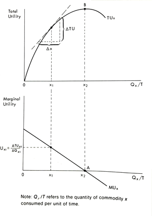
GRAPH 1.1 Total and Marginal
Utility
|
(Kamerschen 72)
|
Graph 1.1 gives a visual explanation of the concepts that
have been discussed, total utility, marginal utility, and the law of
diminishing marginal utility. The TU function starts at 0 and it has a positive
slope until it gets to the maximum, which is labeled B. At B this person does
not get more utility from consuming this product, then the first point in the
MU function has been found. This point is where the MU function is at 0, which
is labeled A. The MU function has a negative slope due to the LDMU. Therefore, it
can be assumed that all the units consumed to the left of point A on the MU
function add value to the TU. (Kamerschen 71)
Consumer
Behavior
Graph 1.2 Equimarginal
principle for a consumer

(Kamerschen 73)
|
In order to understand the consumer behavior, first the
equimarginal principle for a consumer must be understood. The goal of the
equimarginal principle is to balance gains and losses. Marginal benefit (MB) or
marginal utility (MU) equals marginal cost (MC); in the contest of consumers MC
equals price (P). Now let’s look at graph 1.2. The price of a pen equals $1.
This person is willing to pay up to $5 for that first pen, therefore, this
person should continue buying pens until the MC equals the MB which in this
case happens when the fifth pen is bought. (Kamerschen 73)
“The Equimarginal principle says this rule should be applied
to every commodity consumed in order to get optimum division of expenditures”( Kamerschen
74).
(1.2)
Mux/Px=MUy/Py or Mux/MUy= PX/PY
The equation shown on (1.2) says that consumers maximizes
total utility when they are buying the quantities of x and y that allow the MU
per $ spent on x be equal to the MU per dollar spent on y. “Mux/MUy represents
the rate at which the consumer is willing to substitute y for x, and PX/PY represents the rate at which the consumer is
able to substitute y for x. When Mux/Px=MUy/Py is met, the last dollar spent on x
yields the same MU as the last dollar spent on y” (Kamerschen 74).
Table 1.1 Two-good Consumer Optimum,
Marginal Utility Approach

|
(Kamerschen 75)
|
The table 1.1 allows us to visualize the concepts of the equimarginal
principle with a two good situation. The
price of x (Px) equals to $1 and the price of y (Py)
equals to $1, also this consumer has a limited income of $13. To allocate the
money in the best possible way the MUx and MUy for
different quantities of x and y (Qx, Qy) are shown in the
table. Therefore, the buyer will buy the good with the higher MU until he or
she has spent all the income. In this example the consumer will buy 5 units of
x and 8 units of y which both have an equal MU shown at 16 utils (Kamerschen 75).
(1.3) ΔMUy/ΔQx=ΔMUx/ΔQy=
0
(1.4) Mux/Px=MUy/Py=MUz/Pz=…=
λ(common MU per income
dollar)
This “states that the optimum point, marginal utilities must
be in proportion to their prices for all the commodities purchased” (Kamerschen
76).
(1.5) I=Qx
* Px +Qy * Py +Qz *Pz
This “means that the consumer has a budget constraint, so
that total expenditures can not exceed income” (Kamerschen 76)
(1.6) LDMU holds in the case of independent commodities.
This “states that if the commodities are unrelated, the LDMU
must hold” (Kamerschen 77).
Table 1.2 Three-good Consumer
Optimum, Marginal Utility Approach

|
(Kamerschen 78)
|
Table 1.2 allows us to visualize the concepts of the equimarginal
principle with a three good situation. The price of x (Px) equals to
$2, the price of y (Py) equals to $3, and the price of z (Pz)
equals to $1, also this consumer has a limited income of $26. To allocate the
money in the best possible way the MUx, MUy and MUz
(shown on columns 2, 5, and 8) for different quantities of x, y and z (Qx,
Qy, Qz) are shown in the columns (1, 4, and 7). Also the
MU per dollar of each commodity is shown in columns (3, 6, and 9). In order to
find the optimum output, (1.4) and (1.5) must be met. This means that only one
convention of goods (x=2, y=6 and z= 4) will satisfy both (1.4) and (1.5) where
the MU per dollar is equal at 8. There are other conventions that will meet
(1.4) however, not all the income will be spent, which does not meet (1.5) (Kamerschen
76-78).
Derivation of
the Demand
Marshallian Approach
Graph 1.3 Derivation of the
Demand curve (Marshallian)

Market price of P=$2.00 a unit, Pl=$1.50
a unit, Pll=$1.00 a unit
|
(Kamerschen 81)
|
In order to derivate an individual demand curve Dx under
the Marshallian approach the assumption that the MU of money is invariant
(which means that he ignored the income effect) must be done. “Both MUx
and Dx curves measure the Qx on the horizontal axis,
whereas the MU curve measures the MUx on the vertical axis and the
demand curve measures the Px on the vertical axis” (Kamerschen 81). The quantities that the individual buy at
different prices $2.00 a unit, $1.50 a Unit, and $1.00 a unit must be known. The
equation shown in (1.7) shows how to solve for each point in the graph. Since
it is an algebraic equation it can be rewritten as in (1.8). Assuming that the
MU of money
is constant and equal to four utils, and
the Px equal to $2, this consumer will buy 3 units of x because
. This shows that the
consumer will buy 3 units at this price. Therefore, we found our first point in
the demand curve. Then we repeat the process for $1.50 and $1.00 and we find
that at $1.50 the consumer will buy 5 units and at $1.00 will buy 8 units.
(1.7)
Mux/Px
= λ = common MU of money
expenditures
(1.8) Mux=Px
* λ
Walrasian Approach
Graph
1.4 Derivation if the Demand Curve (Walrasian)

“Assuming that price of x is Px1, the price of Y
is Py1 and the respective quantities X1 and Y1.
Also assuming that Px1 is twice Py1, MUx1 must
be twice MUy1. This gives us the first point on the demand curve as
shown on graph 1.4. To find the second point on the demand curve let’s raise
the price of x to Px2, as shown on equation (1.9). We find this is
not at equilibrium any more. Since the price increased the consumer spent more
money on x than y, therefore, the MUy1 increased to MUy2 as
shown in equation (1,10), which tell us that this consumer shifted the money
from x to y. However, this still is not at equilibrium. Since this consumer is
spending more on y the new MUy3 is lower and we find a second point
on the equation as shown in the equation (1.11). A second point on the demand
curve has been established: Px2, X2 (Kamerschen 83-84).
(1.9) Mux1/↑PX2
< MUy1/Py1 so (1.10) Mux1/Px2
< ↑MUy2/Py1 so (1.11) Mux2/Py1=
MUy3/ py1
Consumer and
Producer Surplus
Surplus represents
the fact that consumer and producer’s total economic welfare from the
transaction of a good or service is greater than the utility of its monetary
value (Kamerschen 85).
Marshall Approach of consumer surplus
Assumptions:
is constant there is no income effect
Table 1.3 Calculation of
Consumer Surplus

|
(Kamerschen 86)
|
Graph 1.5 Consumer and
Producer Surplus

|
(Kamerschen 87)
|
Graph 1.5 and
table 1.3 explain the consumer surplus. We can see that for the first unit the
consumer is willing to pay up to $10. At the first unit he has no surplus. For
the second unit he is willing to pay $9. This gives him a $1 surplus. Since the
market price is set at $5 he is willing to buy up to 6 units, which generates a
surplus of $4+ $3 + $2 + $1 or $10. This example deals with discrete
units. If fractional units were not available, the demand curve would be the
step function under Dx
Producer Surplus is analogous to the consumer surplus, which means that
the producer was willing to sell that first unit at a lower price. At the
market price the producer surplus is equal to $9 (Kamerschen 85-87)
Conclusion
Throughout
this document the theory of cardinal utility has been analyzed. This theory
includes the economics concept of total utility (TU), marginal utility (MU),
the law of diminishing marginal utility (LDMU). In addition, this paper
described consumer behavior and the equimarginal principle for a consumer.
Consequently, the Marshalian and Walrasian approach were used to explain the
derivation of the demand curve from the cardinal utility. Finally, this
document explained the consumer and producer surplus concepts.
Work Cited
Kamerschen,
David R, and Lloyd M. Valemtine. Intermediate
Microeconomics Theory. Cincinnati: South-Western Publishing Co, 1977.
Print.
No comments:
Post a Comment